


By Mikko Haapoja and Stephan Leroux
2020 Black Friday Cyber Monday (BFCM) is over, and another BFCM Globe has shipped. We’re extremely proud of the globe, it focused on realism, performance, and the impact our merchants have on the world.
We knew we had a tall task in front of us this year, building something that could represent orders from our one million merchants in just two months. Not only that, we wanted to ship a data visualization for our merchants so they could have a similar experience to the BFCM globe every day in their Live View.
With tight timelines and an ambitious initiative, we immediately jumped into prototypes with three.js and planned our architecture.
Working with a Layer Architecture
As we planned this project, we converged architecturally on the idea of layers. Each layer is similar to a React component where state is minimally shared with the rest of the application, and each layer encapsulates its own functionality. This allowed for code reuse and flexibility to build both the Live View Globe, BFCM Globe, and beyond.
When realism is key, it’s always best to lean on fantastic artists, and that’s where Byron Delgado came in. We hoped that Byron would be able to use the 3D modeling tools he’s used to, and then we would incorporate his 3D models into our experience. This is where the EarthRealistic layer comes in.
EarthRealistic layer from the 2020 BFCM Globe. **EarthRealistic uses a technique called physically based rendering, which most modern 3D modeling software supports. In three.js, physically based rendering is implemented via the MeshPhysicalMaterial or MeshStandardMaterial materials.
To achieve realistic lighting, EarthRealistic is lit by a 32bit EXR Environment Map. By using a 32bit EXR, it means we can have smooth image based lighting. Image based lighting is a technique where a “360 sphere” is created around the 3D scene, and pixels in that image are used to calculate how bright Triangles on 3D models should be. This allows for complex lighting setups without much effort from an artist. Traditionally images on the web such as JPGs and PNGs have a color depth of 8bits. If we were to use these formats and 8bit color depth, our globe lighting would have had horrible gradient banding, missing realism entirely.
Rendering and Lighting the Carbon Offset Visualization
Once we converged on physically based rendering and image based lighting, building the carbon offset layer became clearer. Literally!
Bubbles have an interesting phenomenon where they can be almost opaque at a certain angle and light intensity but in other areas completely transparent. To achieve this look, we created a custom material based on MeshStandardMaterial that reads in an Environment Map and simulates the bubble lighting phenomenon. The following is the easiest way to achieve this with three.js:
- Create a custom Material class that extends off of MeshStandardMaterial.
- Write a custom Vertex or Fragment Shader and define any Uniforms for that Shader Program.
- Override
onBeforeCompile(shader: Shader, _renderer: WebGLRenderer): voidon your custom Material and pass the custom Vertex or Fragment Shader and uniforms via the Shader instance.
Here’s our implementation of the above for the Carbon Offset Shield Material:
- ShieldMaterial.ts - Our custom Carbon Offset Visualization Material
- CustomMeshStandardMaterial.ts - Abstraction on top of MeshStandardMaterial
- shield.frag - Custom Fragment shaders that make MeshStandardMaterial look like a bubble
Let’s look at the above, starting with our Fragment shader. In shield.frag lines 94-97
These two lines are all that are needed to achieve a bubble effect in a fragment shader.
To calculate the brightness of an rgb pixel, you calculate the length or magnitude of the pixel using the GLSL length function. In three.js shaders, outgoingLight is an RGB vec3 representing the outgoing light or pixel to be rendered.
If you remember from earlier, the bubble’s brightness determines how transparent or opaque it should appear. After calculating brightness, we can set the outgoing pixel’s alpha based on the brightness calculation. Here we use the GLSL mix function to go between the expected alpha of the pixel defined by diffuseColor.a and a new custom uniform defined as maxOpacity. By having the concept of min or expected opacity and max opacity, Byron and other artists can tweak visuals to their exact liking.
If you look at our shield.frag file, it may seem daunting! What on earth is all of this code? three.js materials handle a lot of functionality, so it’s best to make small additions and not modify existing code. three.js materials all have their own shaders defined in the ShaderLib folder. To extend a three.js material, you can grab the original material shader code from the src/renderers/shaders/ShaderLib/ folder in the three.js repo and perform any custom calculations before setting gl_FragColor. An easier option to access three.js shader code is to simply console.log the shader.fragmentShader or shader.vertexShader strings, which are exposed in the onBeforeCompile function:
onBeforeCompile runs immediately before the Shader Program is created on the GPU. Here you can override shaders and uniforms. CustomMeshStandardMaterial.ts is an abstraction we wrote to make creating custom materials easier. It overrides the onBeforeCompile function and manages uniforms while your application runs via the setCustomUniform and getCustomUniform functions. You can see this in action in our custom Shield Material when getting and setting maxOpacity:
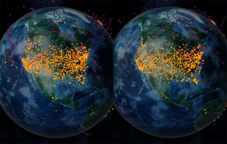
Using Particles to Display Orders
One of the BFCM globe’s main features is the ability to view orders happening in real-time from our merchants and their buyers worldwide. Given Shopify’s scale and amount of orders happening during BFCM, it’s challenging to visually represent all of the orders happening at any given time. We wanted to find a way to showcase the sheer volume of orders our merchants receive over this time in both a visually compelling and performant way.
In the past, we used visual “arcs” to display the connection between a buyer’s and a merchant’s location.

With thousands of orders happening every minute, using arcs alone to represent every order quickly became a visual mess along with a heavy decrease in framerate. One solution was to cap the number of arcs we display, but this would only allow us to display a small fraction of the orders we were processing. Instead, we investigated using a particle-based solution to help fill the gap.
With particles, we wanted to see if we could:
- Handle thousands of orders at any given time on screen.
- Maintain 60 frames per second on low-end devices.
- Have the ability to customize style and animations per order, such as visualizing local and international orders.
From the start, we figured that rendering geometry per an order wouldn't scale well if we wanted to have thousands of orders on screen. Particles appear on the globe as highlights, so they don’t necessarily need to have a 3D perspective. Rather than using triangles for each particle, we began our investigation using three.js Points as a start, which allowed us to draw using dots instead. Next, we needed an efficient way to store data for each particle we wanted to render. Using BufferGeometry, we assigned custom attributes that contained all the information we needed for each particle/order.
To render the points and make use of our attributes, we created a ShaderMaterial, and custom vertex and fragment shaders. Most of the magic for rendering and animating the particles happens inside the vertex shader. Each particle defined in the attributes we pass to our BufferGeometry goes through a series of steps and transformations.
First, each particle has a starting and ending location described using latitude and longitude. Since we want the particle to travel along the surface and not through it, we use a geo interpolation function on our coordinates to find a path that goes along the surface.

Next, to give the particle height along its path, we use high school geometry, a parabola equation based on time to alter the straight path to a curve.

To render the particle to make it look 3D in its travels, we combine our height and projected path data then convert it to a vector position our shader uses as it’s gl_Position. With our particle now knowing where it needs to go, using a time uniform, we drive animations for other changes such as size and color. At the end of the vertex shader, we pass the position and point size to render onto the fragment shader that combines the calculated color and alpha at the time for each particle.
Once the vertex shader is complete, the vertex shader passes position and point size onto the fragment shader that combines the animated color and alpha for each particle.
Given that we wanted to support updating and animating thousands of particles at any moment, we wanted to be careful about how we access and update our attributes. For example, if we had 10000 particles in transit, we need to continue updating those and other data points that are coming in. Instead of updating all of our attributes every time, which can be processor-intensive, we made use of BufferAttribute’s updateRange to update a subset of the attributes we needed to change on each frame instead of the entire attribute set.
Combining all of the above, we saw upwards of 150,000 particles animating to and from locations on the globe without noticing any performance degradation.
Optimizing Performance
In video games, you may have seen settings for different quality levels. These settings modify the render quality of the application. Most modern games will automatically scale performance. Most aggressively, the application may reduce texture quality or how many vertices are rendered per 3D object.
With the amount of development time we had for this project, we simply didn’t have time to be this aggressive. Yet, we still had to support old, low-power devices such as dated mobile phones. Here’s how we implemented an auto optimizer that could increase an iPhone 7+ render performance from 40 frames per second (fps) to a cool 60fps.
If your application isn’t performing well, you might see a graph like this:
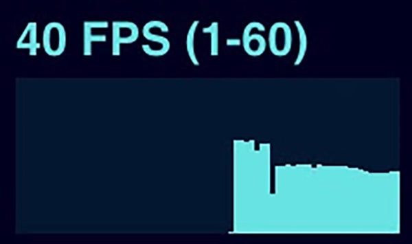
Ideally, in modern applications, your application should be running at 60fps or more. You can also use this metric to determine when you should lower the quality of your application. Our initial implementation plan was to keep it simple and make every device with a low-resolution display run in low quality. However, this would mean new phones with low-resolution displays and extremely capable GPUs would receive a low-quality experience. Our final attempt monitors fps. If it’s lower than 55fps for over 2 seconds, we decrease the application’s quality. This adjustment allows phones such as the new iPhone 12 Pro Max to run in the highest quality possible while an iPhone 7+ can render at lower quality but consistent high framerate. Decreasing the quality of an application by reducing buffer sizes is optimal. However, in our aggressive timeline, this would have created many bugs and overall application instability.
What we opted for instead was simple and likely more effective. When our application retains a low frame rate, we simply reduce the size of the <canvas> HTML element, which means we’re rendering fewer pixels. After this, WebGL has to do far less work, in most cases, 2x or 3x less work. When our WebGLRenderer is created, we setPixelRatio based on window.devicePixelRatio. When we’ve retained a low frame rate, we simply drop the canvas pixel ratio back down to 1x. The visual differences are nominal and mainly noticeable in edge aliasing. This technique is simple but effective. We also reduce the resolution of our Environment Maps generated by PMREMGenerator, but most applications will be able to utilize the devicePixelRatio drop more effectively.
If you’re curious, this is what our graph looks like after the Auto Optimizer kicks in (red circled area)

Globe 2021
We hope you enjoyed this behind the scenes look at the 2020 BFCM Globe and learned some tips and tricks along the way. We believe that by shipping two globes in a short amount of time, we were able to focus on the things that mattered most while still keeping a high degree of quality. However, the best part of all of this is that our globe implementation now lives on as a library internally that we can use to ship future globes. Onward to 2021!
*All data is unaudited and is subject to adjustment.
**Made with Natural Earth; textures from Visible Earth NASA
Mikko Haapoja is a development manager from Toronto. At Shopify he focuses on 3D, Augmented Reality, and Virtual Reality. On a sunny day if you’re in the beaches area you might see him flying around on his OneWheel or paddleboarding on the lake.
Stephan Leroux is a Staff Developer on Shopify's AR/VR team investigating the intersection of commerce and 3D. He has been at Shopify for 3 years working on bringing 3D experiences to the platform through product and prototypes.
Additional Information
three.js
- MeshPhysicalMaterial
- MeshStandardMaterial
- onBeforeCompile
- Points
- BufferGeometry
- ShaderMaterial
- BufferAttribute
- WebGLRenderer
- setPixelRatio
- PMREMGenerator
OpenGL
We're planning to DOUBLE our engineering team in 2021 by hiring 2,021 new technical roles (see what we did there?). Our platform handled record-breaking sales over BFCM, and commerce isn't slowing down. Help us scale & make commerce better for everyone.