A Five-Step Guide for Conducting Exploratory Data Analysis

Have you ever been handed a dataset and then been asked to describe it? When I was first starting out in data science, this question confused me. My first thought was “What do you mean?” followed by “Can you be more specific?” The reality is that exploratory data analysis (EDA) is a critical tool in every data scientist’s kit, and the results are invaluable for answering important business questions.

Simply put, an EDA refers to performing visualizations and identifying significant patterns, such as correlated features, missing data, and outliers. EDA’s are also essential for providing hypotheses for why these patterns occur. It most likely won’t appear in your data product, data highlight, or dashboard, but it will help to inform all of these things.

Below, I’ll walk you through key tips for performing an effective EDA. For the more seasoned data scientists, the contents of this post may not come as a surprise (rather a good reminder!), but for the new data scientists, I’ll provide a potential framework that can help you get started on your journey. We’ll use a synthetic dataset for illustrative purposes. The data below does not reflect actual data from Shopify merchants. As we go step-by-step, I encourage you to take notes as you progress through each section!

Before You Start

Before you start exploring the data, you should try to understand the data at a high level. Speak to leadership and product to try to gain as much context as possible to help inform where to focus your efforts. Are you interested in performing a prediction task? Is the task purely for exploratory purposes? Depending on the intended outcome, you might point out very different things in your EDA.

With that context, it’s now time to look at your dataset. It’s important to identify how many samples (rows) and how many features (columns) are in your dataset. The size of your data helps inform any computational bottlenecks that may occur down the road. For instance, computing a correlation matrix on large datasets can take quite a bit of time. If your dataset is too big to work within a Jupyter notebook, I suggest subsampling so you have something that represents your data, but isn’t too big to work with.

Once you have your data in a suitable working environment, it’s usually a good idea to look at the first couple rows. The above image shows an example dataset we can use for our EDA. This dataset is used to analyze merchant behaviour. Here are a few details about the features:

• Shop Cohort: the month and year a merchant joined Shopify
• GMV (Gross Merchandise Volume): total value of merchandise sold.
• AOV (Average Order Value): the average value of customers' orders since their first order.
• Conversion Rate: the percentage of sessions that resulted in a purchase.
• Sessions: the total number of sessions on your online store.
• Fulfilled Orders: the number of orders that have been packaged and shipped.
• Delivered Orders: the number of orders that have been received by the customer.

One question to address is “What is the unique identifier of each row in the data?” A unique identifier can be a column or set of columns that is guaranteed to be unique across rows in your dataset. This is key for distinguishing rows and referencing them in our EDA.

Now, if you’ve been taking notes, here’s what they may look like so far:

• The dataset is about merchant behaviour. It consists of historic information about a set of merchants collected on a daily basis
• The dataset contains 1500 samples and 13 features. This is a reasonable size and will allow me to work in Jupyter notebooks
• Each row of my data is uniquely identified by the “Snapshot Date” and “Shop ID” columns. In other words, my data contains one row per shop per day
• There are 100 unique Shop IDs and 15 unique Snapshot Dates
• Snapshot Dates range from ‘2020-01-01’ to ‘2020-01-15’ for a total of 15 days

1. Check For Missing Data

Now that we’ve decided how we’re going to work with the data, we begin to look at the data itself. Checking your data for missing values is usually a good place to start. For this analysis, and future analysis, I suggest analyzing features one at a time and ranking them with respect to your specific analysis. For example, if we look at the below missing values analysis, we’d simply count the number of missing values for each feature, and then rank the features by largest amount of missing values to smallest. This is especially useful if there are a large amount of features.

Let’s look at an example of something that might occur in your data. Suppose a feature has 70 percent of its values missing. As a result of such a high amount of missing data, some may suggest to just remove this feature entirely from the data. However, before we do anything, we try to understand what this feature represents and why we’re seeing this behaviour. After further analysis, we may discover that this feature represents a response to a survey question, and in most cases it was left blank. A possible hypothesis is that a large proportion of the population didn’t feel comfortable providing an answer. If we simply remove this feature, we introduce bias into our data. Therefore, this missing data is a feature in its own right and should be treated as such.

Now for each feature, I suggest trying to understand why the data is missing and what it can mean. Unfortunately, this isn’t always so simple and an answer might not exist. That’s why an entire area of statistics, Imputation, is devoted to this problem and offers several solutions. What approach you choose depends entirely on the type of data. For time series data without seasonality or trend, you can replace missing values with the mean or median. If the time series does contain a trend but not seasonality, then you can apply a linear interpolation. If it contains both, then you should adjust for the seasonality and then apply a linear interpolation. In the survey example I discussed above, I handle missing values by creating a new category “Not Answered” for the survey question feature. I won’t go into detail about all the various methods here, however, I suggest reading How to Handle Missing Data for more details on Imputation.

Great! We’ve now identified the missing values in our data—let’s update our summary notes:

• ...
• 10 features contain missing values
• “Fulfilled Orders” contains the most missing values at 8% and “Shop Currency” contains the least at 6%

2. Provide Basic Descriptions of Your Sample and Features

At this point in our EDA, we’ve identified features with missing values, but we still know very little about our data. So let’s try to fill in some of the blanks. Let’s categorize our features as either:

Continuous: A feature that is continuous can assume an infinite number of values in a given range. An example of a continuous feature is a merchant’s Gross Merchandise Value (GMV).

Discrete: A feature that is discrete can assume a countable number of values and is always numeric. An example of a discrete feature is a merchant’s Sessions.

Categorical: A feature that is discrete can only assume a finite number of values. An example of a discrete feature is a merchant’s Shopify plan type.

The goal is to classify all your features into one of these three categories.

GMV	AOV	Conversion Rate
62894.85	628.95	0.17
NaN	1390.86	0.07
25890.06	258.90	0.04
6446.36	64.46	0.20
47432.44	258.90	0.10

 Example of continuous features

Sessions	Products Sold	Fulfilled Orders
11	52	108
119	46	96
182	47	98
147	44	99
45	65	125

 Example of discrete features

Plan	Country	Shop Cohort
Plus	UK	Nan
Advanced Shopify	UK	2019-04
Plus	Canada	2019-04
Advanced Shopify	Canada	2019-06
Advanced Shopify	UK	2019-06

 Example of categorical features

You might be asking yourself, how does classifying features help us? This categorization helps us decide what visualizations to choose in our EDA, and what statistical methods we can apply to this data. Some visualizations won’t work on all continuous, discrete, and categorical features. This means we have to treat groups of each type of feature differently. We will see how this works in later sections.

Let’s focus on continuous features first. Record any characteristics that you think are important, such as the maximum and minimum values for that feature. Do the same thing for discrete features. For categorical features, some things I like to check for are the number of unique values and the number of occurrences of each unique value. Let’s add our findings to our summary notes:

•  ...
• There are 3 continuous features, 4 discrete features, and 4 categorical features
• GMV:
• Continuous Feature
•  Values are between $12.07 and $814468.03
• Data is missing for one day…I should check to make sure this isn’t a data collection error”
•  Plan:
• Categorical Feature
• Assumes four values: “Basic Shopify”, “Shopify”, “Advanced Shopify”, and “Plus”.
• The value counts of “Basic Shopify”, “Shopify”, “Advanced Shopify”, and “Plus” are 255, 420, 450, and 375, respectively
• There seems to be more merchants on the “Advanced Shopify” plan than on the “Basic” plan. Does this make sense?

3. Identify The Shape of Your Data

The shape of a feature can tell you so much about it. What do I mean by shape? I’m referring to the distribution of your data, and how it can change over time. Let’s plot a few features from our dataset:

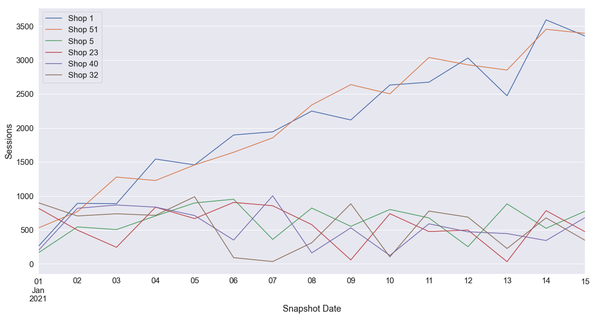
If the dataset is a time series, then we investigate how the feature changes over time. Perhaps there’s a seasonality to the feature or a positive/negative linear trend over time. These are all important things to consider in your EDA. In the graphs above, we can see that AOV and Sessions have positive linear trends and Sessions emits a seasonality (a distinct behaviour that occurs in intervals). Recall that Snapshot Data and Shop ID uniquely define our data, so the seasonality we observe can be due to particular shops having more sessions than other shops in the data. In the line graph below, we see that the Sessions seasonality was a result of two specific shops: Shop 1 and Shop 51. Perhaps these shops have a higher GMV or AOV?

Next, you’ll calculate the mean and variance of each feature. Does the feature hardly change at all? Is it constantly changing? Try to hypothesize about the behaviour you see. A feature that has a very low or very high variance may require additional investigation.

Probability Density Functions (PDFs) and Probability Mass Functions (PMFs) are your friends. To understand the shape of your features, PMFs are used for discrete features and PDFs for continuous features.

Here a few things that PMFs and PDFs can tell you about your data:

• Skewness
• Is the feature heterogeneous (multimodal)?
• If the PDF has a gap in it, the feature may be disconnected.
• Is it bounded?

We can see from the example feature density functions above that all three features are skewed. Skewness measures the asymmetry of your data. This might deter us from using the mean as a measure of central tendency. The median is more robust, but it comes with additional computational cost.

Overall, there are a lot of things you can consider when visualizing the distribution of your data. For more great ideas, I recommend reading Exploratory Data Analysis. Don’t forget to update your summary notes:

• ...
• AOV:
• Continuous Feature
• Values are between $38.69 and $8994.58
• 8% of values missing
• Observe a large skewness in the data.
• Observe a positive linear trend across samples
• Sessions:
• Discrete Feature
• Contains count data (can assume non-negative integer data)
• Values are between 2 and 2257
• 7.7% of values missing
• Observe a large skewness in the data
• Observe a positive linear trend across samples
• Shops 1 and 51 have larger daily sessions and show a more rapid growth of sessions compared to other shops in the data
• Conversion Rate:
• Continuous Feature
• Values are between 0.0 and 0.86
• 7.7% of values missing
• Observe a large skewness in the data

4. Identify Significant Correlations

Correlation measures the relationship between two variable quantities. Suppose we focus on the correlation between two continuous features: Delivered Orders and Fulfilled Orders. The easiest way to visualize correlation is by plotting a scatter plot with Delivered Orders on the y axis and Fulfilled Orders on the x axis. As expected, there’s a positive relationship between these two features.

If you have a high number of features in your dataset, then you can’t create this plot for all of them—it takes too long. So, I recommend computing the Pearson correlation matrix for your dataset. It measures the linear correlation between features in your dataset and assigns a value between -1 and 1 to each feature pair. A positive value indicates a positive relationship and a negative value indicates a negative relationship.

It’s important to take note of all significant correlation between features. It’s possible that you might observe many relationships between features in your dataset, but you might also observe very little. Every dataset is different! Try to form hypotheses around why features might be correlated with each other.

In the correlation matrix above, we see a few interesting things. First of all, we see a large positive correlation between Fulfilled Orders and Delivered Orders, and between GMV and AOV. We also see a slight positive correlation between Sessions, GMV, and AOV. These are significant patterns that you should take note of.

Since our data is a time series, we also look at the autocorrelation of shops. Computing the autocorrelation reveals relationships between a signal’s current value and its previous values. For instance, there could be a positive correlation between a shop’s GMV today and its GMV from 7 days ago. In other words, customers like to shop more on Saturdays compared to Mondays. I won’t go into any more detail here since Time Series Analysis is a very large area of statistics, but I suggest reading A Very Short Course on Time Series Analysis.

Shop Cohort	2019-01	2019-02	2019-03	2019-04	2019-05	2019-06
Plan
Adv. Shopify	71	102	27	71	87	73
Basic Shopify	45	44	42	59	0	57
Plus	29	55	69	44	71	86
Shopify	53	72	108	72	60	28

Contingency table for discrete features “Shop Cohort” an “Plan”

The methodology outlined above only applies to continuous and discrete features. There are a few ways to compute correlation between categorical features, however, I’ll only discuss one, the Pearson chi-square test. This involves taking pairs of discrete features and computing their contingency table. Each cell in the contingency table shows the frequency of observations. In the Pearson chi-square test, the null hypothesis is that the categorical variables in question are independent and, therefore, not related. In the table above, we compute the contingency table for two categorical features from our dataset: Shop Cohort and Plan. After that, we perform a hypothesis test using the chi-square distribution with a specified alpha level of significance. We then determine whether the categorical features are independent or dependent.

5. Spot Outliers in the Dataset

Last, but certainly not least, spotting outliers in your dataset is a crucial step in EDA. Outliers are significantly different from other samples in your dataset and can lead to major problems when performing statistical tasks following your EDA. There are many reasons why an outlier might occur. Perhaps there was a measurement error for that sample and feature, but in many cases outliers occur naturally.

The box plot visualization is extremely useful for identifying outliers. In the above figure, we observe that all features contain quite a few outliers because we see data points that are distant from the majority of the data.

There are many ways to identify outliers. It doesn’t make sense to plot all of our features one at a time to spot outliers, so how do we systematically accomplish this? One way is to compute the 1st and 99th percentile for each feature, then classify data points that are greater than the 99th percentile or less than the 1st percentile. For each feature, count the number of outliers, then rank them from most outliers to least outliers. Focus on the features that have the most outliers and try to understand why that might be. Take note of your findings.

Unfortunately, the aforementioned approach doesn’t work for discrete features since there needs to be an ordering to compute percentiles. An outlier can mean many things. Suppose our discrete feature can assume one of three values: apple, orange, or pear. For 99 percent of samples, the value is either apple or orange, and only 1 percent for pear. This is one way we might classify an outlier for this feature. For more advanced methods on detecting anomalies in categorical data, check out Outlier Analysis.

What’s Next?

We’re at the finish line and completed our EDA. Let’s review the main takeaways:

• Missing values can plague your data. Make sure to understand why they are there and how you plan to deal with them.
• Provide a basic description of your features and categorize them. This will drastically change the visualizations you use and the statistical methods you apply.
• Understand your data by visualizing its distribution. You never know what you will find! Get comfortable with how your data changes across samples and over time.
• Your features have relationships! Make note of them. These relationships can come in handy down the road.
• Outliers can dampen your fun only if you don’t know about them. Make known the unknowns!

But what do we do next? Well that all depends on the problem. It’s useful to present a summary of your findings to leadership and product. By performing an EDA, you might answer some of those crucial business questions we alluded to earlier. Going forward, does your team want to perform a regression or classification on the dataset? Do they want it to power a KPI dashboard? So many wonderful options and opportunities to explore!

It’s important to note that an EDA is a very large area of focus. The steps I suggest are by no means exhaustive and if I had the time I could write a book on the subject! In this post, I share some of the most common approaches, but there’s so much more that can be added to your own EDA.

If you’re passionate about data at scale, and you’re eager to learn more, we’re hiring! Reach out to us or apply on our careers page.

---

Wherever you are, your next journey starts here! If building systems from the ground up to solve real-world problems interests you, our Engineering blog has stories about other challenges we have encountered. Intrigued? Visit our Data Science & Engineering career page to find out about our open positions. Learn about how we’re hiring to design the future together—a future that is Digital by Design.